Machine Learning in Apache Spark Quick Start Guide
Spark Machine Learning
NEW! Spark 3.3 is now available on Qubole. Qubole’s multi-engine data lake fuses ease of use with cost-savings. Now powered by Spark 3.3, it’s faster and more scalable than ever.
In most instances, a Data Scientist will use a notebook to develop a model. Once the model is ready, it can be pre-trained for production serving or deployed to production for regular training.
For example, you might want to re-train your model on a daily basis to improve its accuracy based on a new data, or even implement incremental real-time training.

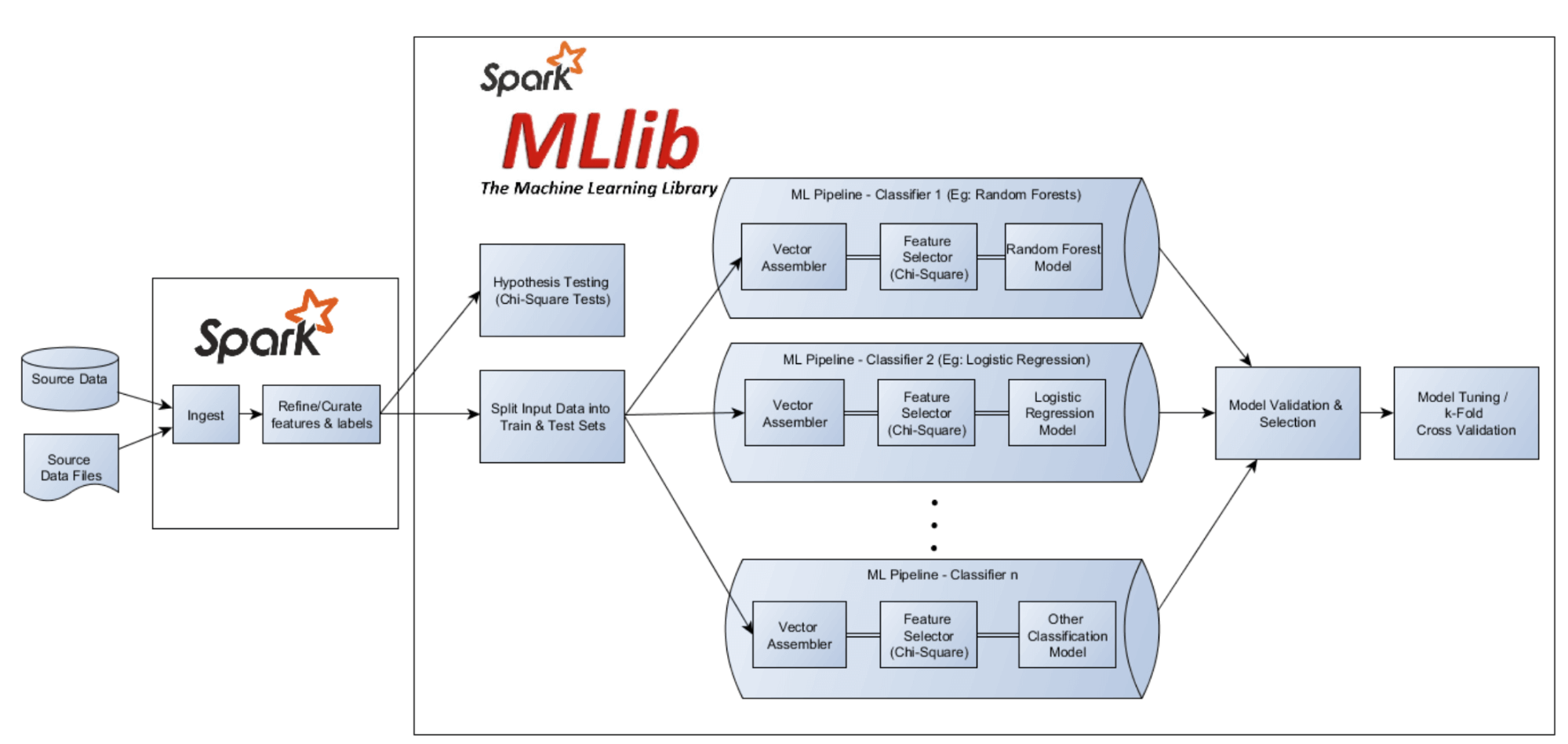
For this example we will be showing the former process, batch model training. We will be using the Customer Churn Prediction Notebook (screen of pipeline above) to cover:
- Data Preparation (for ML training)
- Building ML Pipeline & Feature Engineering
- Training Predictive Model
Data Preparation
As you may remember from the first section, the core foundational building block for Spark is the RDD (Resilient Distributed Datasets), which is essentially a distributed data structure that spans across many computing nodes in the cluster.
While the Spark core aims to analyze the data in distributed memory, there is a separate module in Apache Spark called Spark MLlib for enabling machine learning workloads and associated tasks on massive data sets. With MLlib, fitting a machine learning model to a billion observations can take a couple lines of code and leverage hundreds of machines. MLlib greatly simplifies the model development process.
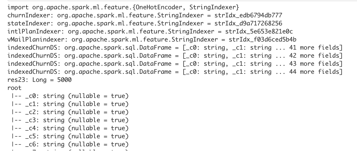
In general, predictive modeling needs String and Category variables to be encoded as numeric values. Using the OneHotEncoder library (provided by MLlib), the code snippet below converts the category variables of the telco dataset into numerically encoded values.
%spark
import org.apache.spark.ml.feature.{OneHotEncoder, StringIndexer}

val churnIndexer = new StringIndexer().setInputCol("churned").setOutputCol("label")
val stateIndexer = new StringIndexer().setInputCol("state").setOutputCol("state_indexed")
val intlPlanIndexer = new StringIndexer().setInputCol("intl_plan").setOutputCol("intl_plan_indexed")
val vMailPlanindexer = new StringIndexer().setInputCol("voice_mail_plan").setOutputCol("voice_mail_plan_indexed")

var indexedChurnDS = churnIndexer.fit(churnsAllDS).transform(churnsAllDS)
indexedChurnDS=stateIndexer.fit(indexedChurnDS).transform(indexedChurnDS)
indexedChurnDS=intlPlanIndexer.fit(indexedChurnDS).transform(indexedChurnDS)
indexedChurnDS=vMailPlanindexer.fit(indexedChurnDS).transform(indexedChurnDS)

indexedChurnDS.count

indexedChurnDS.printSchema
The final display statement results summarize what we accomplished in this step.

Feature Engineering
Now that we have curated our Telco Customer Churn dataset in (distributed) memory and initialized our machine learning pipelines, we will start defining the stages for our ML pipelines.
The first stage of our pipelining process is the feature and label vector creation. for this we will reuse the vectorAssembler object we initialized for observing ChiSquare test results.
Building ML Pipelines
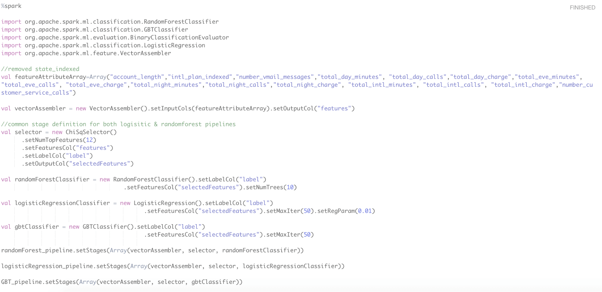
The second stage of our pipelining process is the feature selection stage. Rather than manually inspecting our hypothesis testing results (ChiSquare test results) and selecting the top features (attributes) for our machine learning models, we will define the ChiSqSelector API as a stage and let it automatically perform ChiSquare tests and select the most significant features that influence customer churn.
Notice we are only looking at the top 12 features, given the ChiSquare tests told us we only have 7 very strong influential features, 1 strong, and 4 low correlating features.
The last stage is the final area where the pipeline will be defined by initializing RandomForestClassifier & LogisticRegression API’s.

Training Predictive Model on ML Pipelines
Now that we completed defining and constructing our ML pipelines, it is time to train and prime the predictive modeling pipelines. For this we will split the data set into training and test data sets in 70:30% proportions respectively.
Using the Array command, we can split our test data, to blindfold the pipeline models and validate the results with a clean dataset compared to the predicted churned label on the split data.
%spark
val Array(training, test) = indexedChurnDS.randomSplit(Array(0.7, 0.3))
val randomForestModel = randomForest_pipeline.fit(training)
val logisticRegressionModel = logisticRegression_pipeline.fit(training)
val gbtModel= GBT_pipeline.fit(training)
Proceed to the next section where we will talk about the operational steps in the ML process from selecting our model, going into production, and monitoring.


